Pathfinding, starring Shakey the robot

I’ve mentioned recently how much I enjoy Advent of Code challenges (no spoilers here, don’t worry). One topic I’ve found fascinating is how to write algorithms that find their way around graphs. There’s a lot of history on how people came up with things, and a wide range of problems they can help with (not just Christmas themed made-up puzzles).

This may be a niche topic. Lots of people aren’t too inclined to read about this, and lots of others know much more than me already … I’ll do my best to keep it interesting.

What kind of graph?

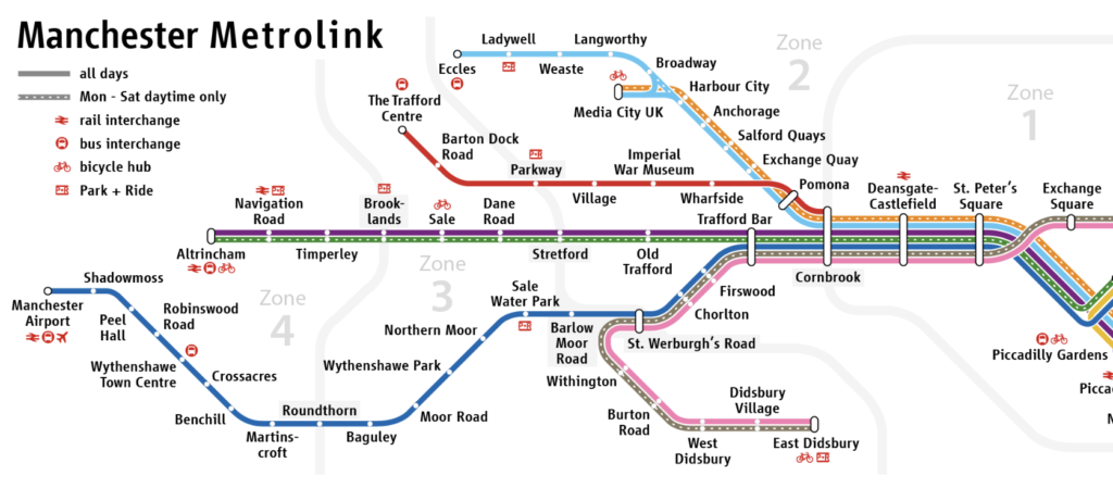
A “graph” in this sense is a collection of nodes (places you can be, also called “vertices”) and edges (connections you can follow to get to other nodes). This abstract description can be applied to lots of things – one example is a tube or tram map.

If you’re at one node (station) on this graph, you can follow the edges (lines) to get to other nodes. A map like this one lets you see what routes you can take.

Some more examples of things you can represent as graphs:

• A satnav can use addresses as nodes and all roads in between them as edges.
• A computer game can model the areas your character can walk to as a “grid” of squares – at each square (node) you can move North, South, East or West to a neighbouring square, assuming there’s no walls or anything blocking your way. The “free to move this way” choices are (very short) edges you can follow.
• A collection of servers (nodes) can be networked together with cables (edges), and data can be sent between them. The Internet uses this graph to route data around different paths if one becomes unavailable.
• Lots of games can be described as graphs – a Rubik’s cube, noughts and crosses, and many more. The node you’re currently at is one state of the game (cube with colours all over the place, or a grid with an X in the middle), each possible move you could make is an edge to follow to a new state. Like searching a map, you can know the goal you’d like to reach and explore how to get there.

You can probably think of a few different things you could use a graph to do:

• Find a good (or the best) way to travel between two nodes on the graph.
• Work out the nearest treasures to your character in a maze, accounting for winding paths and dead ends.
• Work out well-connected things are, so you know there are alternative routes if something goes wrong.
• Think ahead several game moves to decide which choice now might lead to better outcomes later.

The answers to these isn’t always obvious from a glance at the graph; if you’ve ever stood tracing your finger along a tube map, counting stations and changes for different options to get to your destination, you’ll know that “having a graph” can be a bit of work away from “having the answers you want”.

So, who’s this robot?

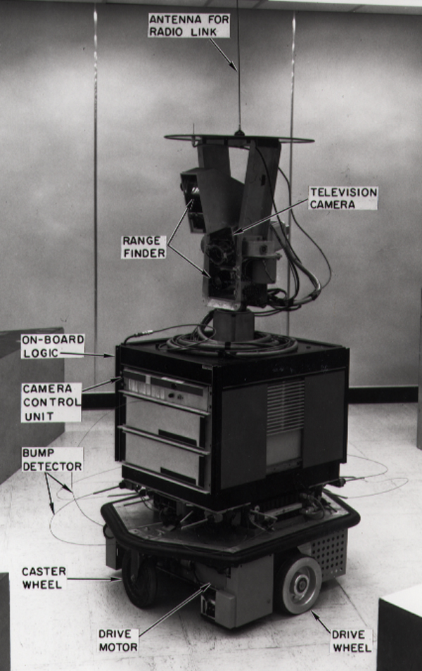
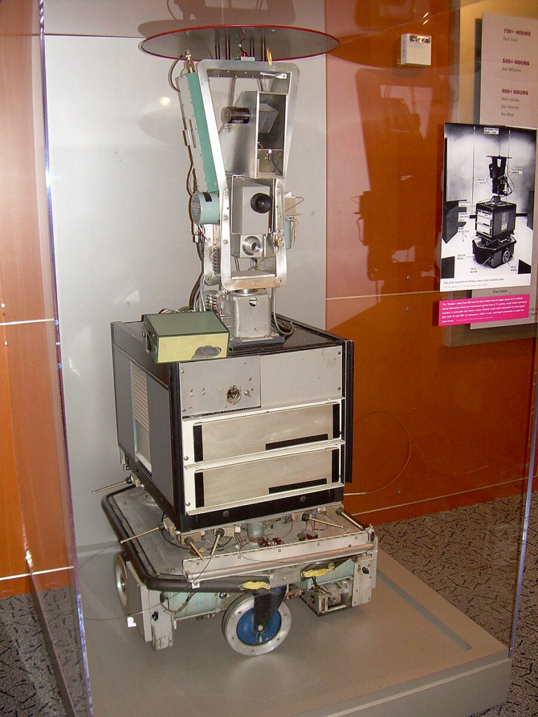
Shakey the robot was built and used in the 1960s and 70s, at the Artificial Intelligence Centre of Stanford Research. It was named because despite the engineers’ best attempts, it kept shaking alarmingly as it moved around the lab.

Shakey’s lab was set up with different rooms and corridors, with objects like blocks, platforms and ramps in them. Shakey could take fairly complex, high-level goals as instructions and work out how to achieve them. To do this, researchers made all kinds of advances in natural language processing, computer vision, and pathfinding. It’s amazing what was achieved so many decades ago. This 1972 video shows Shakey in action. The project was funded by DARPA (part of the US Department of Defense) – you can see where concerns about Terminator-style future robots might come from.

Among the many still-used-today algorithms and techniques that came out of working with Shakey, the A* search algorithm is the one that really caught my eye. This comes up all the time when you look into pathfinding algorithms – it’s key for route planning applications, computer games, and lots of other “what’s the best route from here to there” graph questions. We’ll take a look at how it works in the next part of this post, but first: one more robot fact.

Shakey’s successor was Flakey the robot, I’m not kidding. There’s video of Flakey too.

How some pathfinding algorithms work

I’ve read lots of guides on A* and related algorithms – my current favourite is Amit Patel’s Introduction to the A* Algorithm on the Red Blob Games site. It has interactive animations and guides on how to implement it. If my short descriptions here leave you wanting more detail, I recommend heading there.

There’s a family of related algorithms, starting with breadth-first search. This was invented by Konrad Zuse in 1945, in his PhD thesis – but the thesis got rejected because he forgot to pay a university fee, and his work was fairly unknown for years. This same algorithm got independently invented by Edward F. Moore in 1959.

Breadth-first search cycles round spreading out in all available directions from the starting node, meaning that when you hit the goal node you know there’s no other path that can get there in fewer steps (if you’ve hit it with one path that took 10 steps, you’ve also explored 9 or 10 steps of all other possible paths, so you can stop). A couple of limitations lead to people looking for better goal-finding algorithms:

• This spreads out in all directions equally, so you might do a lot of searching. In small graphs or with close goals this doesn’t matter – just use breadth-first search. Remember, when we talk about the more sophisticated algorithms: they do some extra work so you can avoid doing as much exploring. If there wasn’t much exploring to do in the first place, you might make things worse.
• For finding the shortest path, this can only count the steps. In some graphs, you might want each “step” to have different costs, in which case you’ll need something different.

Edges with costs

When might the “count of steps” not be what matters? How about this graph:

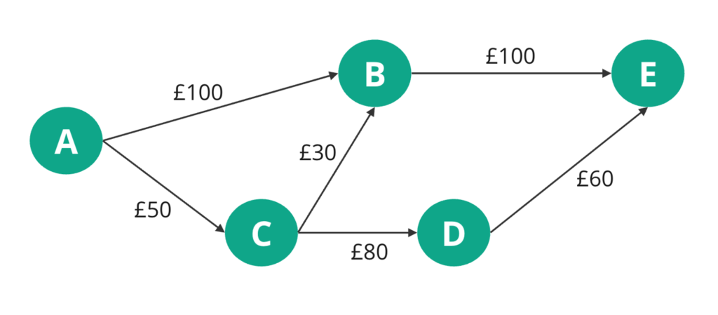
The nodes (with letters) here are airports, and the edges are labelled with the ticket price for each flight. If you wanted to go from A to E, and cared about cost, which route would you take? A→B→E is the shortest number of steps, but there’s definitely cheaper options.

“Cost” doesn’t have to be money:

• For a satnav, you’re mostly concerned with shortest time: If you can drive out of your way a bit to get onto a clear motorway, that’s better than a direct route that goes through city centres.
• For a computer game, you might be concerned about risk: in a stealth mission, some edges might be near enemies or in brightly-lit areas, so you might be seeking the best path for staying hidden.

To solve this problem, Dijkstra’s algorithm has some changes from breadth-first search:

• Instead of the count of steps: track the sum of “costs so far” to get to a node.
• Instead of cycling round edges in the order they’re encountered, making an even spread: keep exploring in whatever direction has the lowest “cost so far”.
• Instead of ignoring already-visited nodes if we find another way to get to them: this way might be a cheaper route, check whether this new “cost so far” should replace the old one.
• Once we find the goal, keep exploring from all nodes that have a lower “cost so far” than the path that’s got us here. If another path is cheaper, switch to that as “best”. Once all other nodes’ costs are above this one, we can stop.

Depending on how many promising paths there are, and how lucky you get by finding one path to the goal early in the search, Dijkstra’s algorithm can cut out quite a bit of searching.

Dijkstra’s “best path” is guaranteed to be the actual best one, so long as none of the edge costs are negative. It’s rare that any will be (maybe … an airline would pay you to fly a certain edge?), but keep it in mind. The problem is that the algorithm might discard a “too expensive” part-finished path, not realising it was about to get cheaper.

This might sound a bit complicated – but it is just a few lines of code different than breadth-first search, which was only about 10 lines to start with. All of these algorithms take some thinking about to understand, but they’re remarkably short to write. Edsger W. Dijkstra claimed that coming up with this one took about 20 minutes, when he was sat outside a cafe – he didn’t have a pencil and paper, which helped force him to keep it simple. Dijkstra invented an amazing range of maths and computing concepts over a long career, and late in life reflected: “Eventually, that algorithm became, to my great amazement, one of the cornerstones of my fame.”

When you know where your goal is

The A* search algorithm builds on Dijkstra’s algorithm. You might notice that breadth-first and Dijkstra’s both spread out without picking a direction. If you know what direction the goal’s in, you can do better.

A* search lets you express which paths are more likely to get us nearer the goal. This can be complicated:

• In a computer game, you might know the exit is to the bottom right of the map, so prefer heading that way. But in a straight line in that direction you might find a wall blocking you, or monsters, so you’d believe a less direct route is needed.
• On a drive from Manchester to Glasgow, you know “North” is the right way to go – but it’s worth considering whether driving South a bit from your start point might be the fastest way to get onto a motorway and cut out a lot of winding traffic. But if you started exploring 50 miles or more South, surely that’s a waste of effort?

A* is exactly like Dijkstra’s algorithm, with the addition of a heuristic. For each step you consider, this heuristic gives an estimated cost to get from there to the goal. This is used:

• When choosing where to explore next, instead of picking the lowest “cost so far”: Pick the lowest “estimated total cost to goal” (that’s “cost so far” (from the start node) plus the “estimated cost from here to goal”).
• Once we find a path to the goal: stop exploring options once their “estimated total cost to goal” is higher than the cost of this path. This can drop options much sooner than Dijkstra’s algorithm, which waits until each option’s “cost so far” is greater than cost of this path.

A* will find the best path, and do so very efficiently – assuming you pick a suitable heuristic function.

• If your estimates are always lower than the actual costs, you’ll get the right answer. The closer to the actual cost your estimate is, the more efficient your search will be – no need to consider lots of other possible paths.
• As your estimates get very low, every option looks promising, and A* will need to keep exploring quite a lot to be sure. At the limit, if your “estimated cost from here to goal” is zero for every question, A* becomes Dijkstra’s algorithm (can only prioritize and discard based on “cost so far”).
• If your estimates perfectly match the actual costs, there’s no exploring to do; A* will march along the best path first time. It’s unlikely you’ll have this!
• If your estimates are higher than the actual costs, you risk throwing away an option that might have been the best path. “I don’t need to look any further along here, it’s going to cost more than the path I found already.”

Picking a suitable heuristic takes some thought and experimentation. A good starting point is: what’s the best this could possibly be? If you’re asked about how long it would take to get from some point to Glasgow, assume the path there is a perfectly straight motorway with no other traffic. I’ve written before about using unreasonable assumptions when estimating – if this impossibly positive assumption still wouldn’t get us there faster than some other path, there’s no need to look into this further. This has the effect of making us explore sooner where that fast finish would be helpful (if we’re asked about somewhere between the start point and Glasgow), and making us put this option far down the list where even being that good wouldn’t help (if we’re asked about somewhere in Cornwall).

Some other “low but still useful” heuristics:

• If you know the exit is down and to the right, using a “straight line from here to there” estimate means nodes roughly between the start and the goal get bumped up the priority list, while others get parked for later and maybe dropped altogether.
• If you’re looking at train costs, maybe you have “some absolute minimum per mile” ticket cost data? Or any other facts that could work out a low-but-useful estimate?

Credit for the A* algorithm goes to Peter Hart, Nils Nilsson and Bertram Raphael, who developed it for Shakey and published it in 1968. There’s a story that they first made an “A1” algorithm, then “A2”, and moved to star to indicate this is the best of all possible version numbers … but I can’t find a good source for that. Let me know if you find any leads on why they picked this name please!

A few more things to think about

Finding the best path between 2 nodes isn’t the only thing you might want to do in a graph – if you want to find all paths, check how connected the graph is, or other jobs, then breadth first search or other algorithms might be your best choice.

I’ve mentioned a few times about keeping things efficient: for smaller, simpler graphs you really won’t notice anything (see “Everything is fast for small n”). But if you have a complicated graph, or if your program needs to check paths a lot, efficiency really starts to matter. Using the right data structures is important: the Wikipedia pages I linked and the Red Blob Games guide I recommended have very helpful implementation examples. I’ve had a go at using these, plus Adrian Mejia’s guide to priority queues, to implement these algorithms in TypeScript in my Advent of Code repo (stick to that one file if you’re avoiding spoilers).

You also need to experiment with any heuristic you’re using for A*: the only thing that’s good for is to help you avoid exploring too much of the graph. A quick-to-calculate, somewhat-accurate heuristic can improve your running time massively. But if calculating the estimates takes more effort than just doing the exploring, you’re not getting any benefit.

If you’re interested in reading more, you might like:

• A very friendly guide to “Big O” notation, a way to understand why some algorithms are faster or far far slower than others: Big O notation basics made dead simple.
• A surprising quiz: Do you know how much your computer can do in a second?
• Stories from a 2015 event celebrating Shakey – looking at how much of an advance that project was, and how much influence it’s had on robotics and AI since: Shakey, from conception to history.